RLP and SSZ: Understanding Serialization Design in Ethereum

This article explores RLP and SSZ, two serialization formats used in Ethereum.Serialization and deserialization are fundamental operations in blockchain protocols, used for tasks such as hash computation, data persistence, and peer-to-peer communication. Rather than relying on general-purpose formats such as Protocol Buffers, Ethereum defines their own serialization rules to reflect their design priorities.In this article, we will examine the specifications and design contexts of RLP and SSZ to understand why they were introduced and what problems they are intended to solve.

RLP

RLP (Recursive Length Prefix) is the encoding method used in the Ethereum execution layer. It is defined in the Ethereum Yellow Paper and has been used since the beginning of Ethereum.

The core idea behind RLP is to encode structured binary data. RLP defines only two data types: byte strings and lists, and the interpretation of those values is left to higher-level protocols. RLP also removes ambiguity from the encoding result, which helps ensure that every machine computes the same hash for the same data. For example, a positive integer is always encoded as the shortest big-endian bytes, and values are encoded explicitly instead of being omitted just because they are zero or otherwise treated as defaults.

Let’s take a deep dive into the specification. RLP encodes data recursively, and each encoded item begins with a prefix byte. There are five possible cases for this prefix byte.

(1) Prefix byte in the range [0x00, 0x7f] → Single Byte

If the data is a single byte with a value less than 0x80, it is encoded as the byte itself.

(2) Prefix byte in the range [0x80, 0xb7] → Short Byte String

If the input is a byte string shorter than 56 bytes, it is encoded as a prefix byte equal to 0x80 + length, followed by the byte string itself.

When a single-byte non-negative integer is encoded in RLP, there are three possible cases. First, the value must be represented as the shortest big-endian byte sequence with no leading zeros. Therefore, if the value is zero, the result will be 0x80, not 0x00, because zero is equivalent to the empty byte string. If the value is in the range [1, 127], it is encoded as the byte itself. Otherwise, it is encoded as a single byte string, prefixed with 0x81 and followed by the byte itself.

(3) Prefix byte in the range [0xb8, 0xbf] → Long Byte String

If the input is a byte string of 56 bytes or more, it is encoded as the concatenation of a prefix, the length of the input, and the input itself. The prefix is 0xb7 + n, where n is the number of bytes in the shortest big-endian representation of the input length with no leading zeros. The encoded input length comes after the prefix, and the input itself follows.

(4) Prefix byte in the range [0xc0, 0xf7] → Short List

If the input is a list whose payload, defined as the concatenation of its encoded items, is less than 56 bytes, it is encoded as a prefix byte followed by the payload. The prefix is 0xc0 + n, where n is the size of the payload.

(5) Prefix byte in the range [0xf8, 0xff] → Long List

If the input is a list whose payload is 56 bytes or more, it is encoded as a prefix byte followed by the payload length and the payload. The prefix is 0xf7 + n, where n is the number of bytes in the shortest big-endian representation of the payload length with no leading zeros.

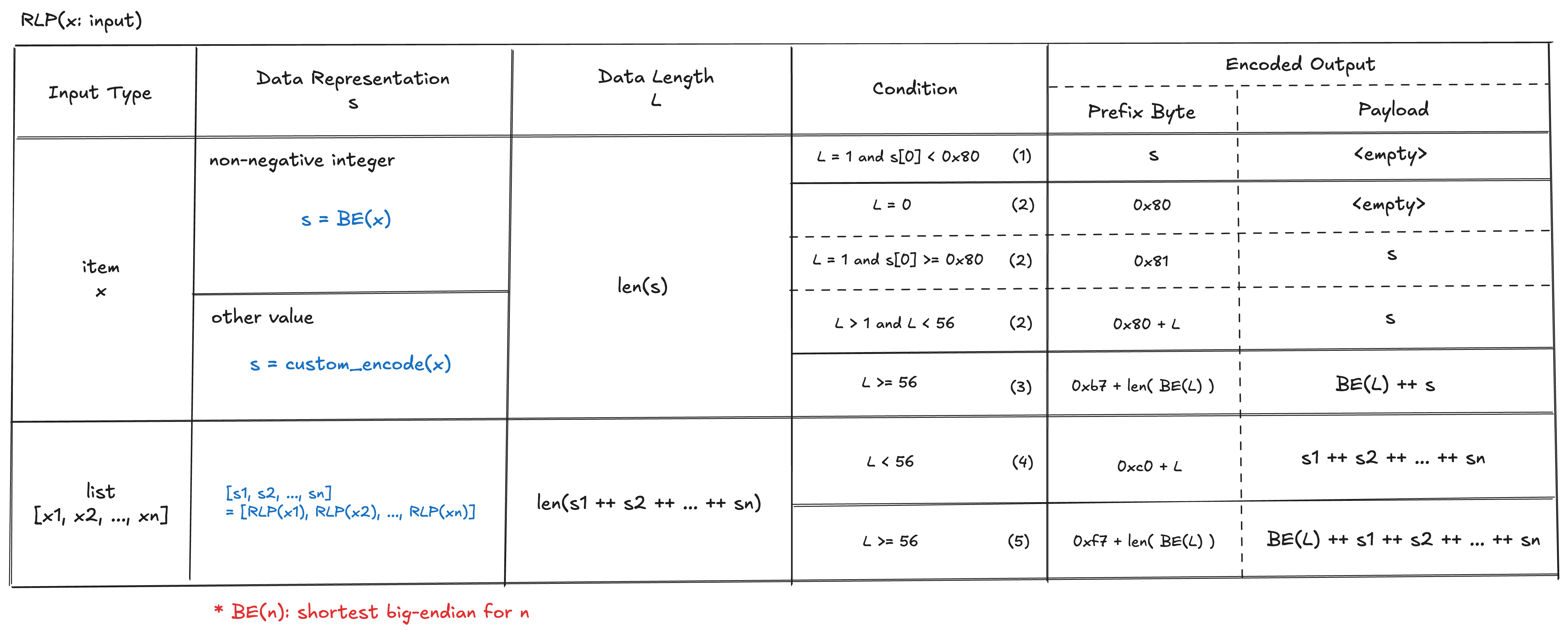
The following table summarizes the full RLP encoding rules.

SSZ

SSZ (Simple SerialiZe) is the serialization format widely used in Ethereum’s consensus layer. One exception is peer discovery, where RLP is still used because the consensus layer relies on discv5, which is also used by the execution layer.

Unlike RLP, SSZ defines a richer set of value types, but its encoding is not self-describing, meaning that the schema must be known in advance for both encoding and decoding. SSZ also defines Merkleization alongside serialization. This unifies data representation and hashing, simplifies implementations, and makes it easier to compute Merkle roots and generate proofs for specific parts of the data.

First, we will examine the SSZ type system and its serialization rules. SSZ data types are classified along two axes: Basic vs. Composite, and fixed-size vs. variable-size. Basic types include only boolean and several unsigned integer types. Composite types represent collections of multiple values, such as list and container (objects). A fixed-size type is a type whose serialized length is known statically, such as boolean values or fixed-length vectors of uint8. All basic types are fixed-size. By contrast, a variable-size type is a type whose serialized length cannot be determined statically, such as a variable-length list of uint8. If a type includes any variable-size data, it is classified as a variable-size type itself.

Basic type serialization

Basic types consist of uint8, uint16, uint32, uint64, uint128, uint256, and boolean, all of which are fixed-size. Each unsigned integer is encoded as its little-endian representation in N/8 bytes, where N is the bit length. With the little-endian encoding SSZ uses, the lower bytes come first, in contrast to RLP, which uses big-endian. For example, consider 399 (0x018f). As a 2-byte integer, it is encoded as 0x01 0x8f in big-endian and 0x8f 0x01 in little-endian. A boolean value is encoded as a single byte: true is serialized to 0x01 and false to 0x00.

Composite type serialization

Composite types represent collections, and include vector, list, bitvector, bitlist, container, and union. Vector and bitvector have a fixed length defined statically in the schema, while list and bitlist are variable-length collections with a maximum length.

Bitvector

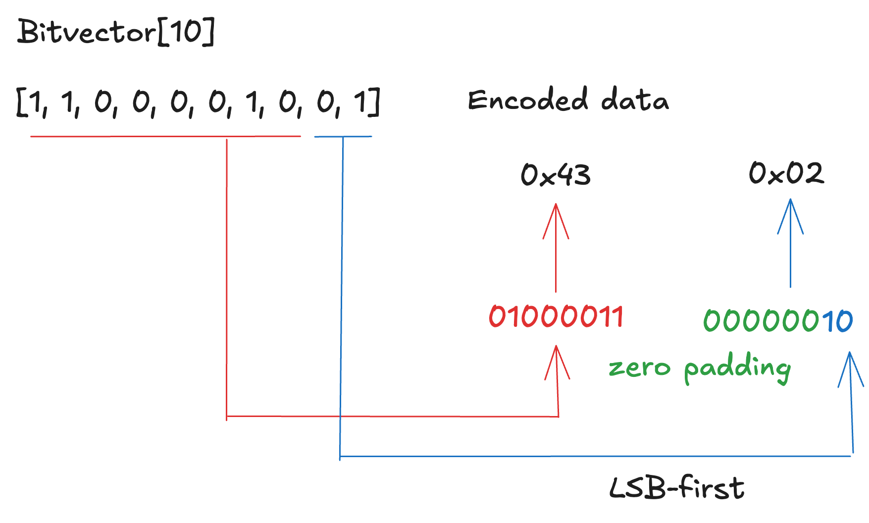
Bitvector is a fixed-size collection of bits. In the spec, it is represented as Bitvector[N], where N is the number of bits. In encoding, bits are packed into ceil(N/8) bytes, meaning the smallest possible number of bytes required to represent N bits. Bits are grouped into bytes of 8 bits each, and earlier bits are placed in the lower-order bit positions within each byte.

For example, the bit sequence [1, 1, 0, 0, 0, 0, 1, 0, 0, 1] is encoded as 0x43 0x02. The first eight bits become 01000011₂, and the remaining two bits become 00000010₂.

Bitlist

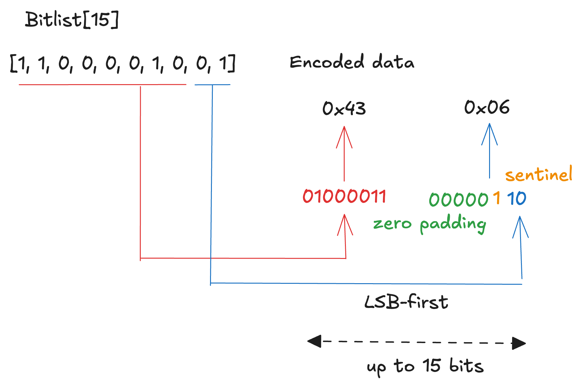
Bitlist is similar to bitvector as a collection of bits, but its length is variable, up to N bits. In the spec, it is represented as Bitlist[N]. The encoding rule is almost the same as bitvector, but 1 is appended after the last element as a sentinel. For this reason, the size of the encoded result is ceil((N+1)/8) bytes.

For example, the bit sequence [1, 1, 0, 0, 0, 0, 1, 0, 0, 1] is encoded as 0x43 0x06. The first eight bits become 01000011₂, and the remaining two bits + sentinel bit become 00000110₂.

Vector, List

Vector and list are collections of elements of a single type. In the specification, they are written as Vector[T, N] and List[T, N]. A Vector[T, N] contains exactly N elements of type T, while a List[T, N] can contain up to N elements of type T.

Vector and list use the same encoding rule, but the encoding depends on the item type. If the item type is fixed-size, the encoded result is simply the concatenation of the encoded items. If the item type is variable-size, the encoded data begins with an array of 32-bit offsets from the beginning of the vector or list, followed by the concatenation of the encoded items.

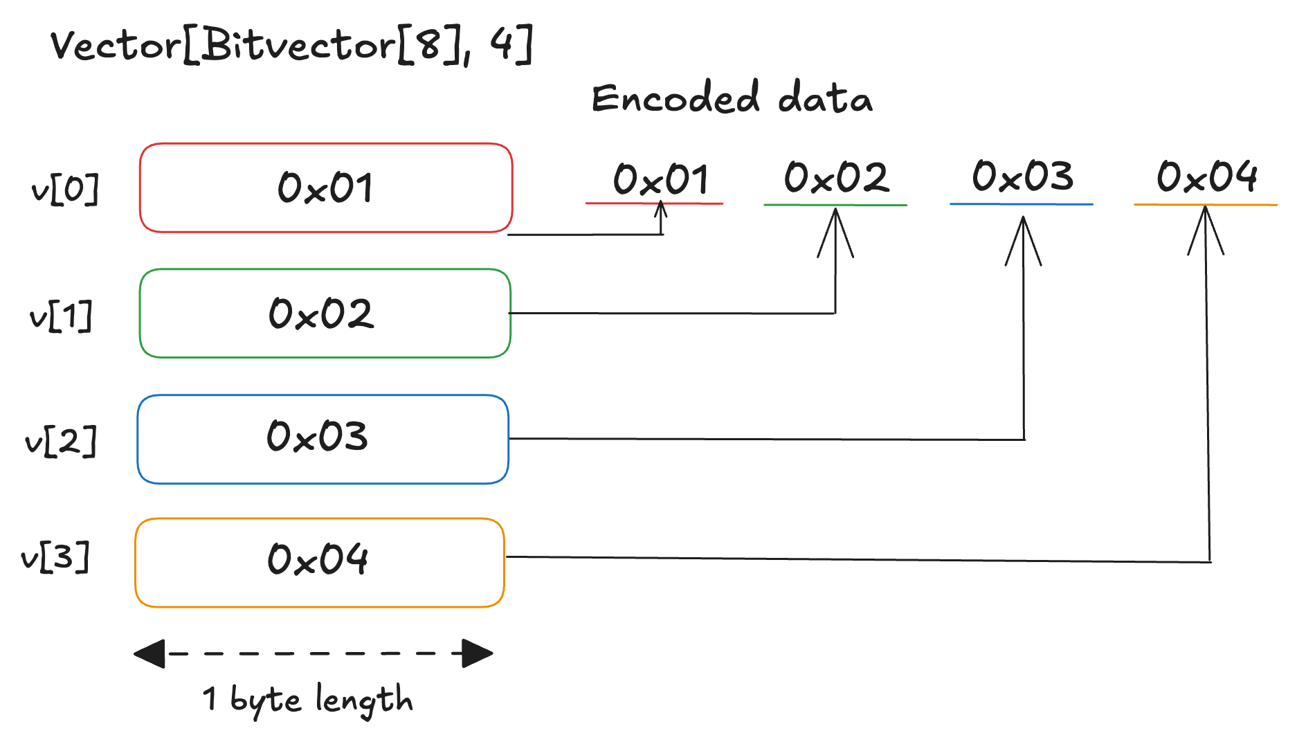
For example, consider encoding [[1,0,0,0,0,0,0,0], [0,1,0,0,0,0,0,0], [1,1,0,0,0,0,0,0], [0,0,1,0,0,0,0,0]] as a Vector[Bitvector[8], 4]. The result is simply the concatenation of each encoded item: 0x01 0x02 0x03 0x04.

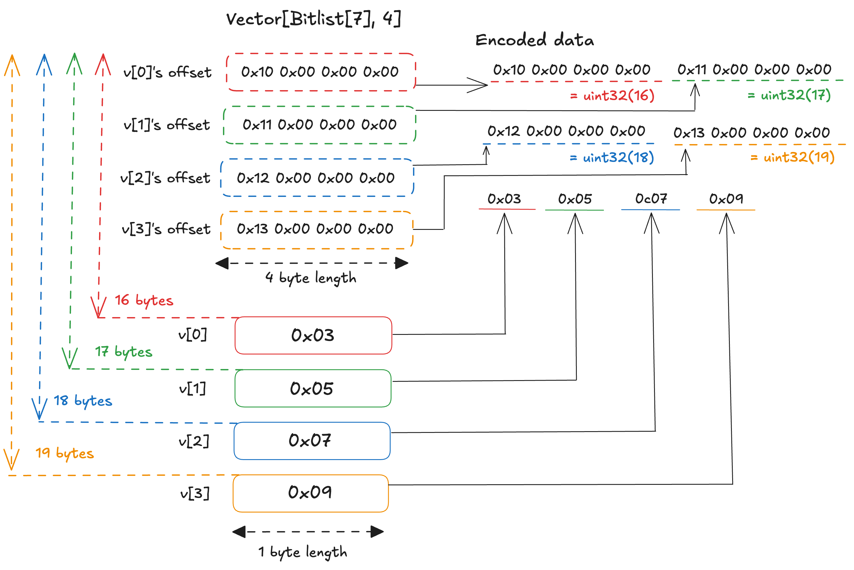
Next, consider encoding [[1], [1, 0], [1,1], [1,0,0]] as Vector[Bitlist[7], 4], where each element contains 1, 2, 2, and 3 bits of data respectively. Each element is encoded by packing the data bits into a byte in LSB-first order, then appending a sentinel bit 1 immediately after the last data bit. The four elements are thus encoded as 0x03, 0x05, 0x07, and 0x09. Since Bitlist is a variable-size type, the vector is encoded by placing the offsets first and the encoded items afterward. Each offset is a little-endian uint32, so the payload begins at byte 16. The offsets are therefore 16, 17, 18, and 19, encoded respectively as 0x10 0x00 0x00 0x00, 0x11 0x00 0x00 0x00, 0x12 0x00 0x00 0x00, and 0x13 0x00 0x00 0x00. The full encoded result is thus 0x10 0x00 0x00 0x00 0x11 0x00 0x00 0x00 0x12 0x00 0x00 0x00 0x13 0x00 0x00 0x00 0x03 0x05 0x07 0x09.

Container

Container is an ordered collections of elements with multiple types. In the spec, a container type is defined using an object-style notation as follows:

class Data(Container):
  key: Vector[uint8, 2]
  credentials: List[uint8, 8]
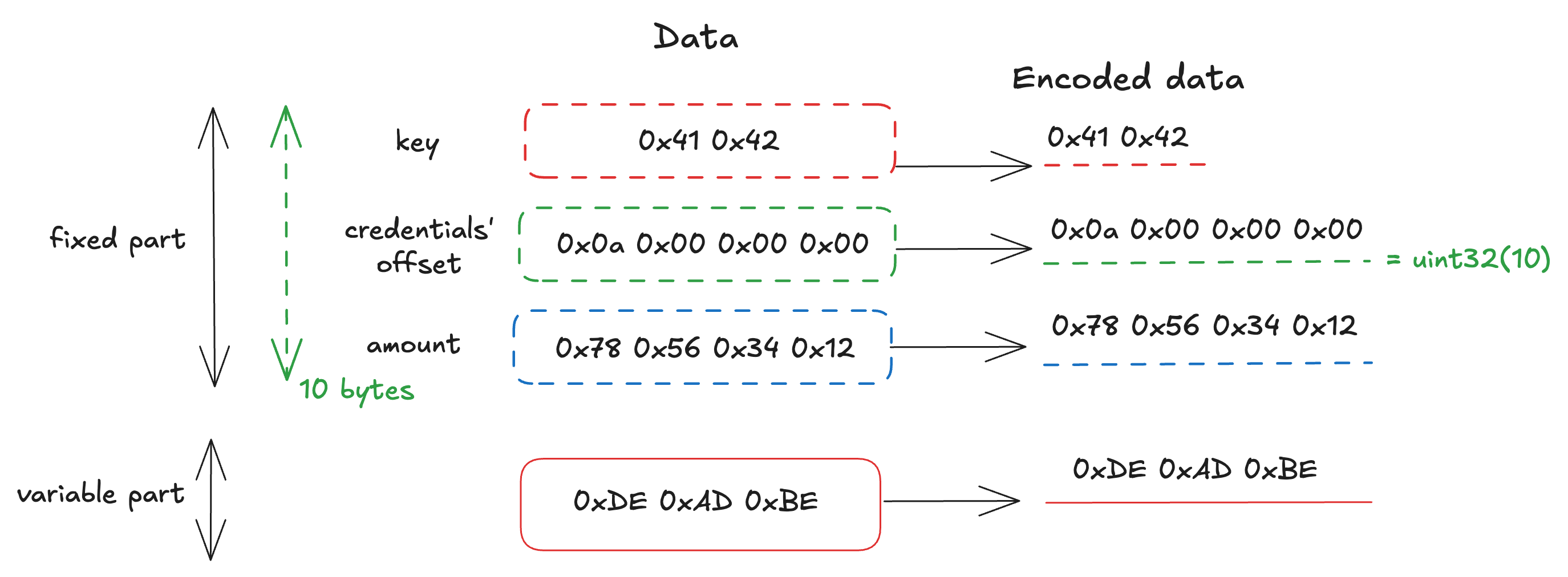
  amount: uint32

The encoding rule for container is the same as for vector and list, and only field values are encoded. However, since a container may include both fixed-size and variable-size fields, the first part of the encoding result consists of the fixed-size values and the offsets for the variable-size fields in order, followed by the variable-size values themselves.

The following figure illustrates the encoding of the data below, based on the schema above.

Data(
    key         = Vector[uint8, 2]([0x41, 0x42]),
    credentials = List[uint8, 8]([0xDE, 0xAD, 0xBE]),
    amount      = uint32(305419896)
)

Union

The SSZ specification also defines unions, but they are not currently used. This article skips the details about unions, but they are used to represent a value that can be one of multiple types.

Alias

The specification also defines several alias types, which are treated as distinct types even though they map to the following underlying types:

• bit → boolean
• byte → uint8
• BytesN → Vector[byte, N]
• ByteVector[N] → Vector[byte, N]
• ByteList[N] → List[byte, N]

Merkleization

SSZ defines Merkleization in addition to serialization, which makes partial proofs possible without revealing the whole structure.

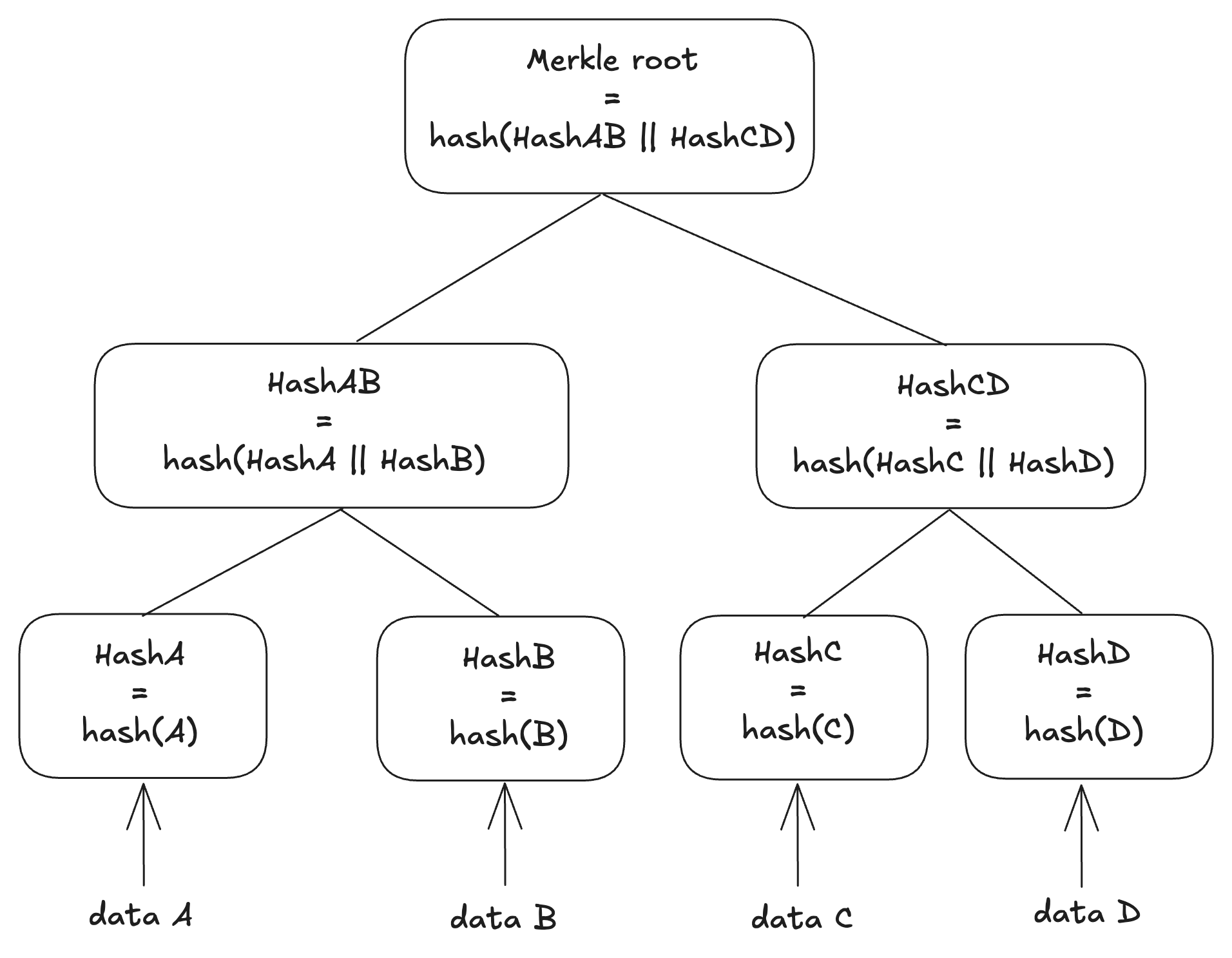
In general, a Merkle tree is a complete binary tree used to compute a single hash commitment over data composed of multiple values. The leaves are hashes of the underlying data, and each internal node is computed by hashing the concatenation of its two children. This structure enables efficient partial verification and compact integrity checks for large datasets.

In SSZ, the hashing rules are defined separately for each data type, and the resulting hashes are computed recursively. However, collections of basic types (e.g. List[uint32, 16]) are first packed into 32-byte chunks, and the Merkle root is computed over those chunks. The tree is always padded to a power-of-two number of leaves, with any remaining slots filled with zero chunks. To distinguish between actual zero data and zero padding, the number of items is included in the hash calculation for variable-length collection types such as List and Bitlist.

Let’s now examine the hashing rules in detail. The specification defines several helper functions used in Merkleization:

• size_of(B) returns the number of bytes required for the given basic type. For example, size_of(uint16) = 2
• chunk_count(T) returns the number of 32-byte chunks required for the given type. It returns the following values:
  • All basic types: 1
  • Bitlist[N] and Bitvector[N]: ceil(N / 256)
  • List[B, N] and Vector[B, N], where B is a basic type: ceil((N * size_of(B)) / 32)
  • List[C, N] and Vector[C, N], where C is a composite type: N
  • Container: the number of fields
• pack(values) creates 32-byte chunks from the given basic type values. It serializes each value, concatenates them in order, right-pads with zeros until the total size is a multiple of 32 bytes, and splits the result into 32-byte chunks.
• pack_bits(bits) creates 32-byte chunks from Bitvector[N] or Bitlist[N]. It removes the sentinel bit for Bitlist, concatenates the bits into a byte string, and passes it to pack(data) to produce 32-byte chunks.
• next_pow_of_two(i) returns the smallest power of two greater than or equal to i, with 0 mapping to 1. This determines the number of leaves required in a complete binary tree for N chunks of data.
• merkleize(chunks, limit) calculates the Merkle root of the given chunks. The limit is an optional value that fixes the tree depth to match the maximum capacity of the type. If limit is provided and less than len(chunks), an error is raised. Otherwise, the chunks are padded with zero-byte chunks to a power-of-two number of leaves next_pow_of_two(limit) if a limit is given, or next_pow_of_two(len(chunks)) if not.
• mix_in_length(root, length) returns hash(root || length), where length is the little-endian serialization of a uint256. This includes the collection size in the hash to distinguish actual data from zero padding.

The merkleization function hash_tree_root(value) is defined for each type as follows:

(1) Value is a basic type

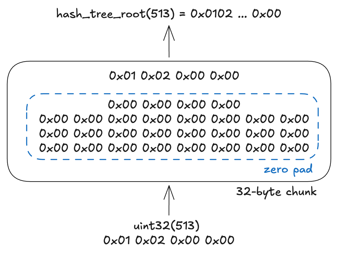
A basic value always fits into a single chunk, so hash_tree_root simply returns the value right-padded with zeroes to 32 bytes.

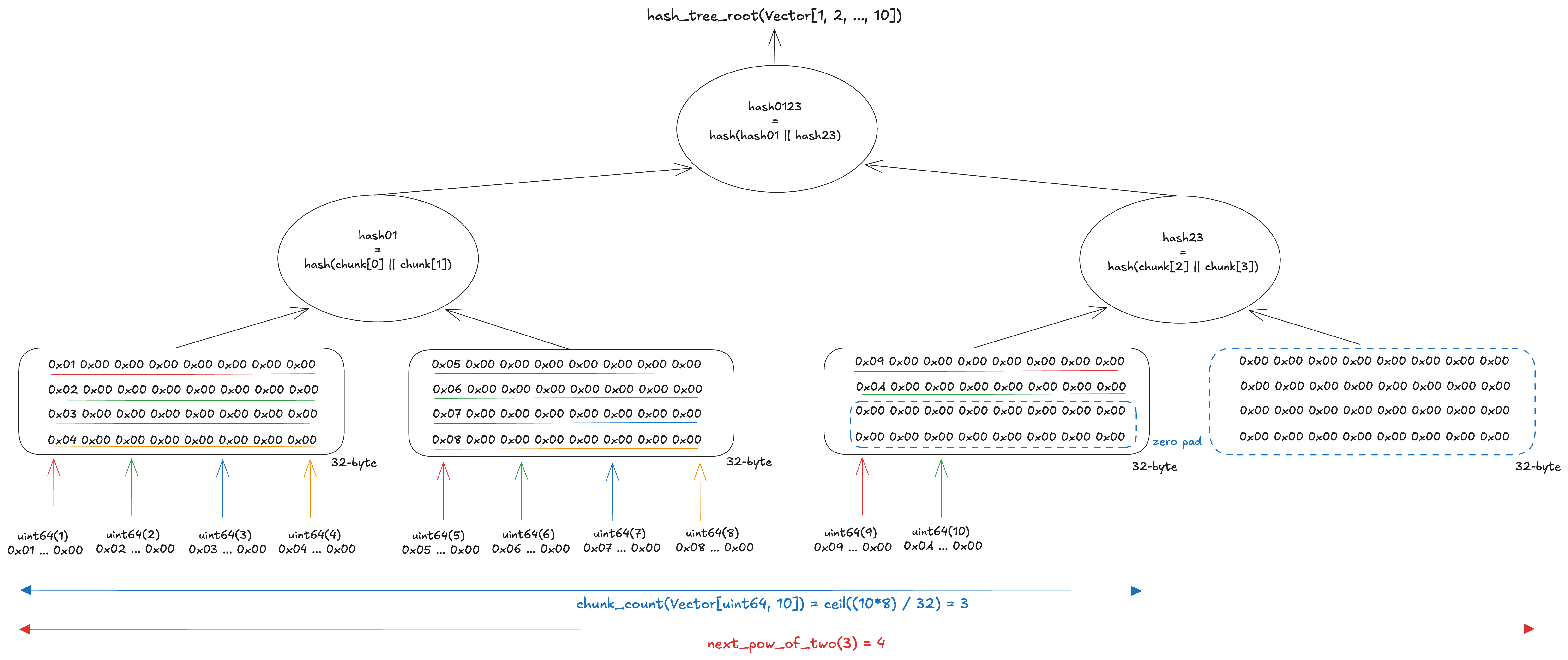
(2) Vector of basic type / Bitvector[N]

If the value is a vector of a basic type, the elements are first serialized and concatenated in order. The result is then zero-padded until the total size reaches n * 32 bytes, where n is chunk_count(T). The data is then split into 32-byte chunks, and the Merkle root is calculated from them.

The figure below shows the calculation of the Merkle root of Vector[uint64, 10]. The total data size is 80 bytes, so 3 chunks of 32 bytes are needed to fit the data. The number of leaves is rounded up to 4, the next power of two after 3. The data is serialized and concatenated into 80 bytes, then zero-padded to 96 bytes (32 bytes × 3) to fill the third chunk. Since next_pow_of_two(3) = 4, one additional zero chunk is appended to reach a power-of-two number of leaves. The data is thus split into 4 chunks of 32 bytes, and the Merkle root is computed from them.

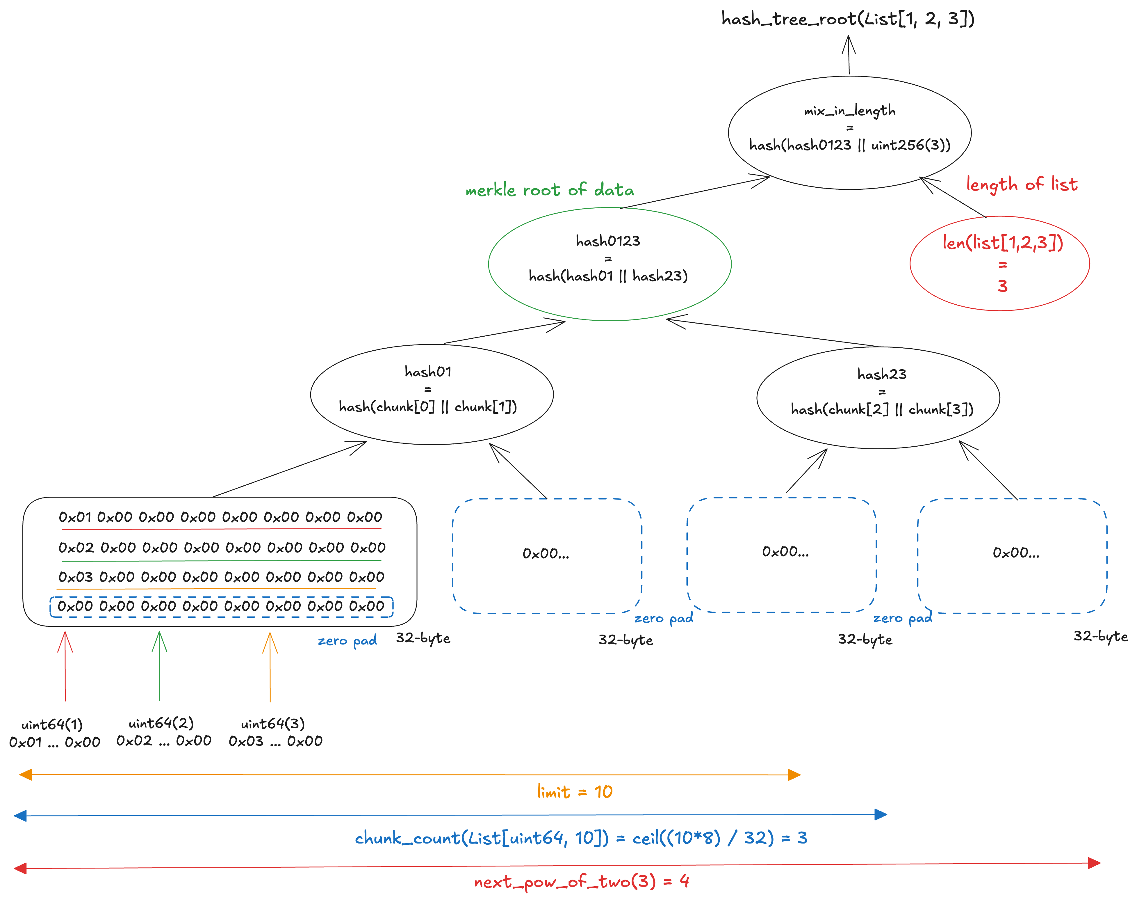
(3) List of basic type / Bitlist[N]

For Lists of basic types or Bitlists, the computation is similar to that of Vectors of basic types or Bitvectors, but there are two key differences:

• The Merkle tree of the data is constructed based on the limit N, not the actual data size
• The Merkle root is computed using mix_in_length, which hashes the Merkle root of the data together with the number of items.

If the tree size were based on the current number of items, the tree depth could change as items are added. In addition, to distinguish between actual zero data and zero padding, the item count is mixed in via mix_in_length

The figure below shows the calculation of the Merkle root of [1, 2, 3] in List[uint64, 10]. The three elements fit into a single chunk, but chunk_count(List[uint64, 10]) = ceil((10×8)/32) = 3, so the tree is built with next_pow_of_two(3) = 4 leaves. The remaining three leaves are filled with zero chunks. The final Merkle root is then computed by hashing the concatenation of the data’s Merkle root and the item count via mix_in_length.

Similarly, for Bitlist[N], the computation is based on the Merkle root of a complete binary tree that can hold N bits, combined with the current bit count via mix_in_length.

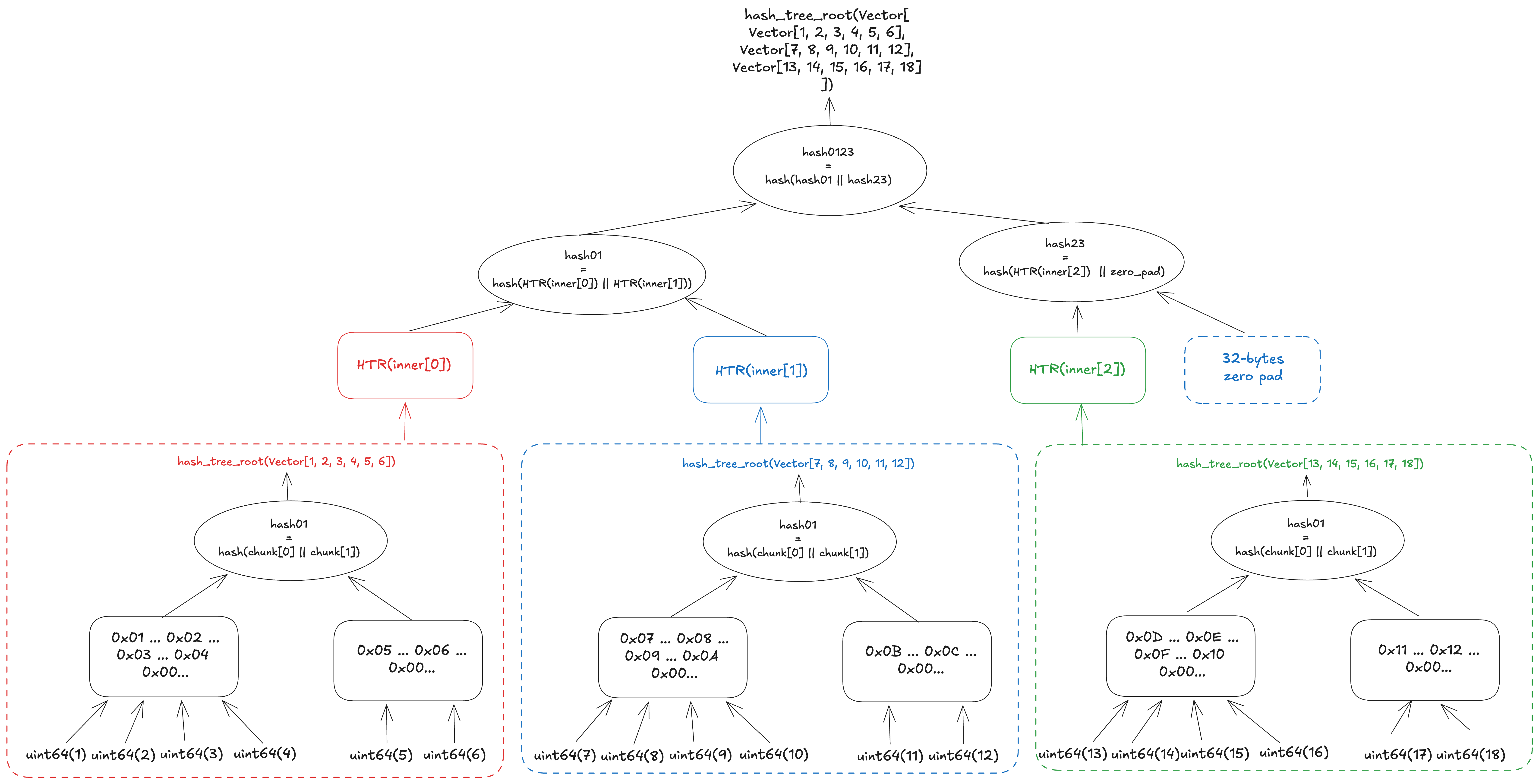
(4) Vector of composite type

For Vectors of composite types, the hash tree root is computed from a tree whose leaves are the hash_tree_root of each element.

The figure below shows the calculation of the hash tree root of Vector[Vector[uint64, 6], 3]. First, the hash tree root is calculated for each inner vector, and then the hash tree root of the outer vector is calculated from a tree whose leaves are the resulting hashes.

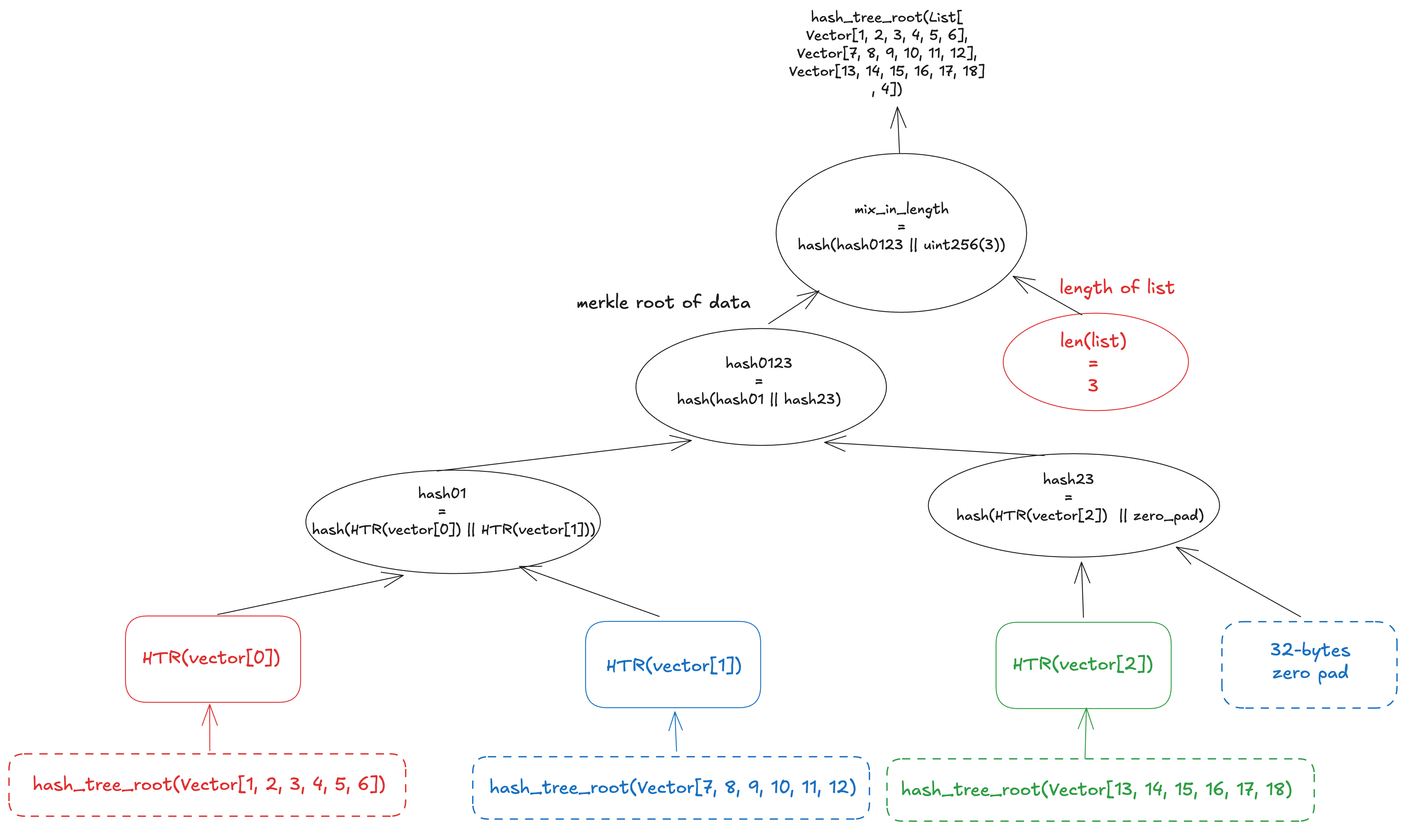
(5) List of composite type

For lists of composite types, the hash tree root is calculated by combining the patterns described above: it is computed from a tree whose leaves are the hash_tree_root of each element, using limit=N to fix the tree depth based on the maximum capacity, and then mixed with the actual number of elements via mix_in_length.

(6) Container

For containers, the hash tree root is calculated from a merkle tree whose leaves are the hash_tree_root of each field. This means basic values are not packed into chunks, unlike in vectors or lists of basic types.

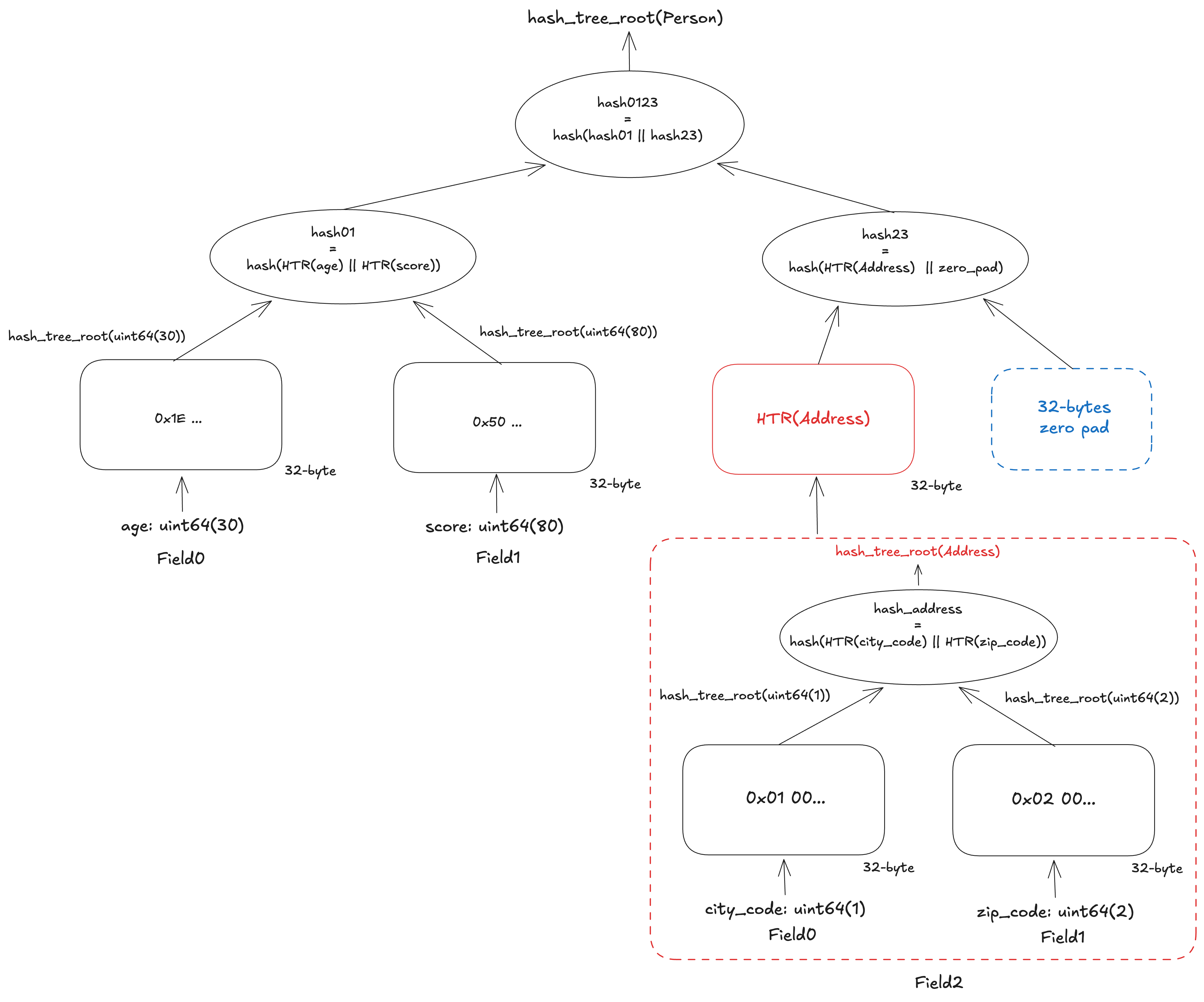
The figure below shows the calculation of the hash tree root of Person. The type definition of Person is as follows:

class Person(Container):
    age:     uint64
    score:   uint64
    address: Address
 
class Address(Container):
    city_code: uint64
    zip_code:  uint64

For the calculation, hash_tree_root is first called for each field. Let’s take a look at the computation for Address first. This container has only 2 basic-type fields, so the tree has 2 leaves. Each leaf contains the 32-byte zero-padded representation of each field: city_code and zip_code. The values are not concatenated but individually padded with zero bytes. The hash tree root of Address is the hash of these 2 leaves.

After calculating Address, we can now compute the hash tree root of Person. This container has 3 fields, so the number of leaves is rounded up to 4. The last leaf will be zero-padded. As with Address, a leaf for a basic-type field is simply the value zero-padded to 32 bytes, while a leaf for a composite-type field is the result of its hash_tree_root.

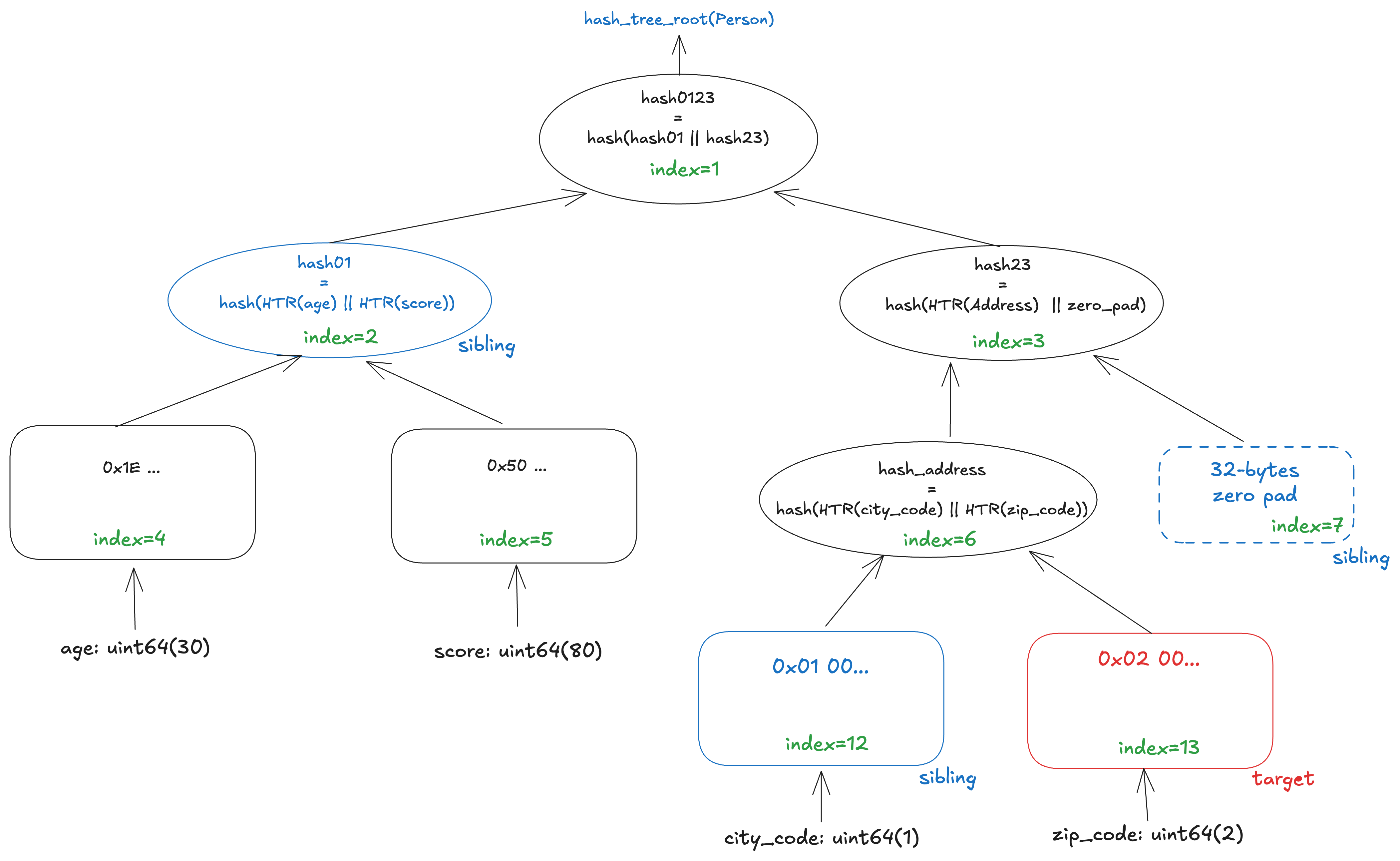
Generalized index

As we have seen, the computation of the hash_tree_root of SSZ data is based on a binary tree. Any node can be identified by its generalized index, no matter how complex the schema is. The rule is simple: the root is 1, the left child of a node k is 2k, and the right child is 2k + 1. With this numbering scheme, each node in the Merkle tree can be referenced by a single integer. A generalized index can be determined statically from the schema alone, without needing the actual data. This is useful when requesting a Merkle proof to verify the inclusion of a specific value.

The figure below illustrates a Merkle proof for zip_code in the SSZ tree of Person. The leaf for zip_code is located at generalized index 13. To prove its inclusion, the prover provides the nodes highlighted in red and blue. These are the values needed to reconstruct the path from zip_code to the root: the target leaf itself and the sibling nodes at indices 12, 7, and 2. By hashing these nodes upward in order, the verifier can recompute hash_tree_root(Person). If the recomputed root matches the expected root, the verifier can confirm that zip_code is part of the original SSZ object.

Summary

RLP and SSZ are two serialization formats used in Ethereum. Rather than adopting existing general-purpose formats, Ethereum introduced its own encodings to prioritize simplicity, schema definitions that closely mirror the specification, and deterministic behavior across implementations. Compared with RLP, SSZ has a richer design. That added complexity, however, brings meaningful benefits: offsets support partial decoding, and standardized Merkleization enables field-level proofs. Together, these features allow consistent and verifiable behavior across a wide range of clients, from full nodes to light clients running on constrained devices.

References

• https://ethereum.github.io/yellowpaper/paper.pdf
• https://ethereum.org/developers/docs/data-structures-and-encoding/rlp
• https://github.com/ethereum/consensus-specs/blob/v1.3.0/ssz/simple-serialize.md
• https://eth2book.info/capella/part2/building_blocks/ssz/#overview
• https://blog.ethereum.org/2014/02/09/why-not-just-use-x-an-instructive-example-from-bitcoin